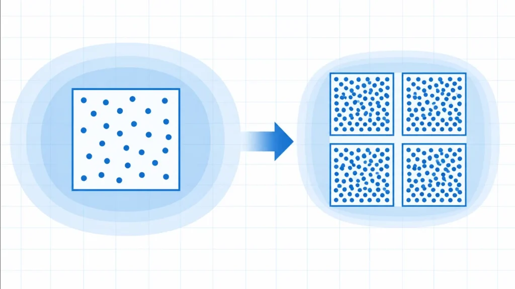
Halving a survey’s margin of error usually requires about four times the sample size because random sampling error shrinks with the square root of the sample size. If 1,000 independent responses support a 3% margin under fixed assumptions, about 4,000 responses support a 1.5% margin.
The four-times rule describes precision from random sampling. It assumes the same confidence level, the same estimate of population variability, and a comparable sampling design. Change one of those conditions, and the required sample size can change for reasons besides the margin of error.
This article explains the square-root relationship, works through several comparisons, and shows where the shortcut needs care. For an exact planning estimate, use the sample size calculator with the assumptions that match your study.
Why Does Precision Improve By The Square Root?
Sampling uncertainty gets smaller as the sample grows, but it does not shrink in direct proportion to the number of observations. Under a simple random sampling model, the standard error contains the sample size under a square root. That makes the margin of error proportional to 1 divided by √n.
Margin of error E = critical value × standard error
For a population proportion, a common planning form is E = z × √[p(1 − p) ÷ n]. The symbol z represents the chosen confidence level, p represents the expected proportion, and n represents the sample size. The same square-root pattern appears in many estimates of a population mean.
Penn State’s lesson on sampling and confidence explains how a sample statistic estimates a population parameter and why repeated random samples vary. That sampling variation is the uncertainty that a confidence interval and its margin of error summarize.
The square root creates diminishing returns. Multiplying n by four divides the standard error by √4, which is two. Multiplying n by nine divides it by √9, which is three. Simply doubling the sample divides the margin by √2, or about 1.414, not by two.
Why does each new response help less than the last? Independent observations add information, but random positive and negative deviations partly balance. The scale of that remaining random variation grows like √n, while the average divides the total by n. Together, those effects produce 1/√n.
How Does Halving The Margin Of Error Require Four Times The Sample?
Start from E proportional to 1/√n and hold every other factor fixed. If the new target margin is half the old one, then the square root of the sample must double. Squaring that change makes the required sample four times as large.
n₂ = n₁ × (E₁ ÷ E₂)²
Suppose a survey design needs 1,000 completed responses for a 3% margin of error. The new goal is 1.5%. The margin ratio is 3 ÷ 1.5 = 2. Square that ratio to get 4, then multiply 1,000 × 4 = 4,000 responses.
| Starting sample | Old margin | New margin | Multiplier | New sample |
|---|---|---|---|---|
| 1,000 | 3% | 1.5% | (3 ÷ 1.5)² = 4 | 4,000 |
| 1,000 | 3% | 2% | (3 ÷ 2)² = 2.25 | 2,250 |
| 1,000 | 3% | 1% | (3 ÷ 1)² = 9 | 9,000 |
The relationship works in either direction. If a completed survey of 4,000 has a 1.5% margin under the model, reducing the sample to 1,000 doubles the margin to 3%. The smaller sample has one-quarter as many observations but twice the random uncertainty, not four times.
You can compare other goals with the same ratio formula. Cutting a 4% margin to 3% needs (4 ÷ 3)², or about 1.778 times the original sample. A study with 900 responses would therefore need about 1,600 responses under the same assumptions.
What Must Stay Fixed For The Four-Times Rule To Work?
The shortcut works only when the confidence level, expected variability, population definition, and sampling design remain comparable. The formula isolates the effect of changing E. If another input changes at the same time, the sample can rise or fall for a second reason.
A higher confidence level uses a larger critical value. Moving from a lower confidence level to a higher one widens the interval unless the sample also grows. You can compare those settings with a confidence interval calculator instead of applying the four-times rule alone.
Variability also matters. For a proportion, p(1 − p) is largest when p = 0.5, so planners often use 0.5 when no reliable prior estimate exists. A proportion expected near zero or one has less model-based variance and may require fewer responses for the same absolute margin.
For a mean, the population standard deviation plays a similar role. A more variable outcome needs a larger sample to reach the same margin. If the standard deviation estimate changes between plans, the margin ratio by itself does not explain the new sample requirement.
OpenStax’s discussion of statistical inference and confidence intervals connects sample estimates, standard error, confidence levels, and interval width. Its framework helps separate the desired precision from the assumptions used to estimate that precision.
How Should You Calculate And Round A Required Sample?
Calculate with the full ratio, then round the final required sample upward to a whole response. Rounding down can leave the planned margin slightly wider than the target. A study cannot collect a fraction of a completed independent observation.
Suppose 750 responses support a 4% margin and the new goal is 3%. Compute 750 × (4 ÷ 3)² = 750 × 1.7777… = 1,333.33…. Round up to 1,334 completed responses.
Plan for completed responses, not invitations. If only part of the contacted group responds, the number invited must be larger than the required analytic sample. For example, expecting 40% completion would require dividing the needed completions by 0.40. That response assumption is operational, not part of the square-root precision rule.
Keep percentages in the same form within the ratio. You may use 4 and 3, or 0.04 and 0.03, because the units cancel. Do not mix 4 with 0.03. That would create a ratio 100 times too large before squaring.
When Does Population Size Change The Calculation?
For a very large population, required sample size depends much more on precision than on the population count. When a simple random sample covers a meaningful share of a finite population without replacement, a finite population correction can reduce the required sample.
Penn State’s sampling-theory guidance gives both the finite-population sample-size formula and the large-population approximation. The finite formula includes the population count N, while the approximation drops that correction when it can reasonably be ignored.
Imagine surveying a school with only 1,200 eligible students. A plan that treats the population as effectively infinite might request a sample approaching or exceeding much of that population. The finite correction recognizes that observing a large fraction of all students leaves less uncertainty about the remaining students.
The usual four-times comparison is most accurate when both sample plans are small relative to the same population. As the new sample becomes a large fraction of the population, the corrected relationship bends. Four times the uncorrected sample may be unnecessary or impossible because the population itself is limited.
A census is the limiting case: if you accurately observe every unit in the defined population, there is no random sampling error from selecting only some units. Measurement error, missing answers, and coverage problems can still remain. Population size does not erase those non-sampling errors.
What Problems Cannot Be Solved By A Larger Sample?
A larger sample reduces random sampling error under the model, but it does not automatically remove bias. Poor question wording, undercoverage, nonresponse, faulty measurements, duplicated records, or a nonrepresentative selection process can produce a precise estimate of the wrong value.
Suppose an online poll collects 100,000 voluntary responses from visitors to one website. Its large count may create a narrow formula-based margin, yet visitors who choose to answer may differ from the target population. The extra responses repeat the same selection problem instead of repairing it.
Nonresponse creates a similar risk when respondents differ systematically from people who do not answer. Sending more invitations can increase the number of completed surveys, but the final sample can remain biased if the response pattern stays uneven.
Better planning begins with a clear target population, a defensible way to reach its members, reliable measurements, and procedures that limit missing data. Sample size supports those choices. It cannot substitute for them.
How Does Dependence Reduce Effective Sample Size?
The square-root rule assumes observations contribute roughly independent information. When responses are strongly related, the effective sample size can be smaller than the head count. Four thousand correlated observations may provide less precision than four thousand independent observations.
The CDC’s NHANES reliability guidance defines effective sample size as the actual sample size divided by the design effect for a complex survey estimate. It also explains that the design effect compares design-based variance with the variance from a simple random sample.
Cluster sampling illustrates the issue. Students from the same classroom may share instruction, location, schedules, and background factors. Their answers can be more alike than answers from students selected independently across many schools. Adding more students within one classroom may add less information than adding students from new classrooms.
Repeated measurements on the same person are also dependent. Ten readings from each of 100 people do not automatically equal 1,000 independent people. A suitable analysis must account for the within-person relationship before it reports uncertainty.
Survey planners often use a design effect to compare a complex design with simple random sampling. A design effect greater than one means more actual observations are needed to achieve the precision of the smaller independent sample. The appropriate value depends on the design and correlation pattern, so it should come from defensible prior data or specialist planning.
How Can You Apply The Rule Safely?
Use the four-times rule as a comparison tool, then check every assumption behind it. The relationship is valuable because it shows the cost of precision quickly. It is not a complete sampling plan.
- Write the current sample size and current margin of error.
- Choose the new absolute margin using the same units.
- Calculate n₂ = n₁ × (E₁ ÷ E₂)².
- Round the final requirement upward.
- Confirm that confidence level and variability stayed fixed.
- Check whether a finite population correction applies.
- Adjust for clustering, dependence, or unequal weighting when needed.
- Plan enough invitations to reach the required completed sample.
Finally, separate precision from study quality. Ask whether the sampling frame covers the target population, whether nonresponse could be uneven, and whether the measurement is valid. A narrow interval is useful only when the data collection process supports the population claim.
Browse the statistics and probability hub for related tools. The key memory aid is simple: margin of error changes with the inverse square root of sample size. Halve the margin, square the factor of two, and expect about four times as many independent observations under fixed assumptions.